Prime partners exist: progress toward the twin prime problem
David W. Farmer
Number theorists view the integers as a largely unexplored landscape populated
by interesting and friendly inhabitants. The prime numbers: 2, 3, 5, 7, 11, 13,...;
occur like irregular mileposts stretching off to infinity. The squares: 1, 4, 9, 16, 25,...;
and the cubes: 1, 8, 27, 64, 125,...; along with the higher powers are more sparse,
but they also demand attention because of their special form.
These intriguing features exist because of the interaction between addition and multiplication.
If we knew only about addition then the integers would be quite boring: start with 0,
then repeatedly add or subtract 1 to get everything else. End of story.
Things become interesting when you add multiplication to the mix.
To construct every integer from addition, all you need is 1.
For multiplication, the prime numbers are the building blocks and
there are infinitely many of them. Examining the list of prime numbers
reveals both structure and apparent randomness. Fairly often (8 times
before 100, and 35 times before 1000) primes occur as "twins,"
meaning that both $p$ and $p+2$ are prime. Examples are 101 and 103,
or 8675309 and 8675311. Somewhat less often, a prime is of the form $n^2+1$,
such as $17=4^2+1$ or $90001 = 300^2+1$.
It is an unsolved problem to determine whether there
are infinitely many primes of the form $p+2$ or $n^2+1$,
where we use $p$ to represent a prime number and $n$ to represent
a positive integer (which may or may not be prime).
Other special forms
which also are unresolved are Mersenne primes ($2^p-1$) and Sophie Germain
primes ($2p+1$). Such problems have been the subject of thousands of
research papers over the past several centuries. And while none have
been solved (nor are they likely to be solved in the near future) a large number
of tools have been developed which have led to partial results.
Recently Yitang Zhang of the University of New Hampshire
has combined several of those tools
to make impressive progress on the twin
prime problem. Below we discuss some variations of these difficult
problems and then describe Zhang's result.
1. Relaxing the conditions: measuring progress on difficult problems
How can one measure progress toward an unsolved problem? One view
when dealing with primes of a special form is to make the form less
restrictive. For example, instead of looking for primes of the form
$n^2+1$, one could ask for primes of the form $n^2+a$, where $a$ is as
small as possible.
Or one could look for primes of the
form $n^2+m^2$, or more ambitiously $n^2+m^4$.
These problems vary widely in difficulty. Fermat proved
that there are infinitely may primes of the form $p=n^2+m^2$, in fact
those are exactly the primes $p\equiv 1 \bmod 4$.
In 1997 John Friedlander and Henryk Iwaniec proved that $n^2+m^4$ is prime infinitely
often, using sieve techniques originally developed by Enrico Bombieri.
A measure of the difficulty of that result is that only
$X^{\frac34}$ of the numbers less than $X$ have that form.
Shortly after, Roger Heath-Brown proved that the even thinner set
$n^3+2m^3$ is prime infinitely often.
One might have suspected that those results would be more difficult than
the twin prime problem, because, by the prime number theorem, there are $X/\log(X)$ numbers of the form
$p+2$ less than $X$, and the naive guess would be that having more
candidates would make the problem easier.
One can generalize the twin prime problem to ask whether $p$ and $p+4$,
or $p+6$, or $p+8$, etc., are prime. This is sometimes called
the "prime neighbors" problem: show that there is some fixed number $2n$ so that
$p$ and $p+2n$ are prime infinitely often. That is exactly the problem which Zhang
recently solved. We describe some of the heuristics behind twin primes and
related problems, and then discuss the techniques behind Zhang's proof.
2. Prime heuristics: the frequency to special primes
Why should we expect to have infinitely many twin primes?
The prime number theorem, proven in 1896 by Haramard and de la Valée-Poussin(sp),
says that the number of primes up to $X$ is asymptotically $X/\log(X)$.
Equivalently, the $n$th prime is asymptotic to $n\log(n)$. Here, and throughout
number theory, "$\log$" means natural logarithm.
By the prime number theorem,
among numbers of size $n$ the primes have density $1/\log(n)$.
This suggests what is known as the "Cramér model" of the
primes: the probability that the large number $n$ is prime is $1/\log(n)$, and
distinct numbers have independent probabilities of being prime.
Thus, the Cramér
model says that the probability that $p$ and $p+2$ are both prime is
$1/\log(p) \cdot 1/\log(p+2) \approx 1/\log^2(p)$, so up to $X$ the Cramér
model predicts approximately $X/\log^2(X)$ twin primes. In particular, there
should be infinitely many of them.
Of course that argument has to be wrong, because it predicts exactly the same answer
for $p$ and $p+1$ being prime -- but that almost never happens because if $p$
is odd then $p+1$ is even.
Hardy and Littlewood, using their famous circle method, developed precise
conjectures for the number of twin primes as well as a wide variety of other
interesting sets of primes. The result is that (in most cases) the Cramér
model predicts the correct order of magnitude, but the constant is wrong.
Using the twin prime case as an example, the idea is that the likelihood of
$p+2$ being prime has to be adjusted based on the fact that $p$ is prime.
If $p$ is odd then $p+2$ also is odd, so there is a $\frac12$ chance
that $p$ and $p+2$ are both odd, which is twice as likely as the Cramér model would predict.
Similarly, we need neither $p$ nor $p+2$ to be a multiple of 3, which happens $\frac13$
of the time -- exactly when $p\equiv 1\bmod 3$. The Cramér model would have that
happen $(\frac{2}{3})^2$ of the time, so we must adjust the probability to
make it slightly
less likely
that $p$ and $p+2$ are prime. Making a similar adjustment
for the primes 5, 7, 11, etc.,
we arrive at the Hardy-Littlewood twin prime conjecture:
$$
\#\{p < X \ :\ p \ \mathrm{ and } \ p+2 \ \text{ are prime } \}
\sim 2 \prod_{p>2} \left( 1- \frac{2}{p}\right) \left(1- \frac{1}{p}\right)^{-2} \cdot \frac{X}{\log^2(X)} .
$$
The twin primes have been tabulated up to $10^{16}$ and so far the Hardy-Littlewood
prediction has been found to be very accurate.
Other prime neighbors, $p$ and $p+2n$, can actually occur more frequently than
the twin
primes. For example, if $p$ is a large prime then $p+6$ is not divisible by
2 or 3, so it is more likely than $p+2$ to be prime. Specifically,
in the case of $p$ and $p+2$, we must have $p\equiv 2 \bmod 3$,
while in the case of $p$ and $p+6$ we
can have $p\equiv 1 \text{ or } 2 \bmod 3$.
Thus, a prime gap of 6 is twice as likely as a prime gap of 2.
The same argument shows that a prime gap of 30 is $\frac83$ times as likely
as a prime gap of 2.
The Hardy-Littlewood method also makes predictions for the frequency
that $n^2+1$, or other polynomials, represent primes.
All those conjectures are also supported
by numerical observations.
Precise predictions supported by data are nice, but it is better to have an actual proof.
The methods for proving results about primes of a special form involve the ancient
idea of a prime sieve. The appendix has information about the archtypal
sieve of Eratosthenes.
3. Sieving for primes
For twin primes, the first nontrivial result was due to Viggo Brun
in 1915, using what is now known as the Brun sieve. Brun
proved that there are not too many twin primes. In particular,
Brun proved that
$$
\sum_{p, p+2, \text{ prime}} \frac{1}{p} < \infty.
$$
This is consistent with the Hardy-Littlewood conjecture because
$\sum 1/n\log^2(n)$ converges. Since $\sum_p 1/p$ diverges,
which was proven by Euler and also follows from the prime number
theorem, we see that most prime numbers are not twin primes.
This is a negative result, in terms of our goal of showing
that there are infinitely many twin primes.
To state things positively, we wish to find a parameter $A$
such that for infinitely many $p$ there exists $a\le A$ with
$p+a$ prime. By the prime number theorem, the average
distance between a prime $p$ and the next prime is $\log(p)$,
so we can take $A=\log(p)$. It is nontrivial to show $A=C\log(p)$
for some fixed number $C< 1$. The existence of such a number $C$ was
first proven by Hardy and Littlewood in 1927, assuming the Generalized
Riemann Hypothesis. An unconditional proof was given by Erdős
in 1940, using the Brun sieve. Erdős' result did not provide
a specific value for $C$; this was remedied by Ricci in 1954,
who found $C\le \frac{15}{16}$. Bombieri and Davenport modified the
Hardy-Littlewood method to make it unconditional (and better!),
obtaining
$C\le \frac12$. Various subsequent improvements in the years up to 1988
led to $C\le 0.2484...$.
The next big development, which is one of the main ingredients
in Zhang's recent work, is due to Goldston, Pintz, and Yıldırım,
in 2005.
For the rest of this article
we will refer to the method of those three authors as "GPY."
It is GPY, combined with some techniques from the 1980's, which made
Zhang's result possible. All the GPY papers are in the AIM preprint series,
available at {\tt http://aimath.org/preprints.html}.
The GPY method uses a variant of the Selberg sieve to prove that $A=C \log(p)$
for any $A>0$, and later improved this to
$$
\phantom{x}\ \ \ \ \ \ \ \ \ \ \ \ \ \ \ \
A=\sqrt{\mathstrut \log(p)} (\log\log(p))^2.
\ \ \ \ \ \ \ \ \ \ \ \ \ \ \ \
(1)
$$
The method also shows that if the primes have
"level of distribution $\vartheta>\frac12$," the precise meaning of which
is described below, then one could find an absolute bound for $A$,
independent of $p$. The GPY method was the topic of the November, 2005,
AIM workshop
Gaps between primes. One highlight of the workshop was
Soundararajan presenting a proof that $\vartheta=\frac12$ is the true obstruction
for the GPY method to produce bounded gaps between primes.
An intetresting sidelight is that the workshop was the first occasion that
Goldston, Pintz, and Yıldırım were all in the same place at the same time.
4. Primes in progressions: a tool for optimizing the sieve
Key to the GPY method is knowledge about the distributions of primes in
arithmetic progressions. If $a$ and $q$ are integers with no common factor,
then Dirichlet proved that there are infinitely many primes
$p\equiv a \bmod q$. For example, 4 and 15 have no common factor,
so the sequence
$$
4, 19, 34, 49, 64, 79, ...
$$
contains infinitely many primes. In 1899, de la Valée-Poussin went further, showing that
all such progressions contain the expected number of primes.
Here "expected" means that each of the progressions $\bmod\ q$ that can contain infinitely
many primes, asymptotically contains the same number of primes. To continue our
previous example of progressions $\bmod 15$, there are 8 possible choices
for the number $a$: 1, 2, 4, 7, 8, 11, 13, and 14. Every large prime
has one of those numbers as its remainder when divided by 15, and all
8 remainders occur equally often. The number of possible remainders $\bmod q$
is denoted by the Euler phi-function, $\varphi(q)$, so $\varphi(15)=8$.
The general case is that if $a$ and $q$ have no common factors, then
$$
\sum_{\ontop{p< x}{p\equiv a \bmod q}} \log(p)
\ \ \ \ \ \ \
\text{ is asymptotic to }
\ \ \ \ \ \ \
\frac{x}{\varphi(q)}.
$$
de la Valée-Poussin actually did a bit better,
providing a main term and an explicit error term.
5. Level of distribution: how well we can control the primes
A shortcoming of the above results is that they only hold for fixed $q$ as $x\to\infty$.
For the GPY mythod, and the subsequent work of Zhang, one requires $q$ to grow with $x$,
and allowing $q$ to grow faster gives better results. To describe the
issue more precisely,
we introduce the "error" term
$$
E(x; q, a) = \left|\sum_{\ontop{p< x}{p\equiv a \bmod q}} \log(p) - \frac{x}{\varphi(q)}\right|.
$$
For applications, we would like $E(x; q, a)$ to be small when $q=x^\alpha$ for
$\alpha$ as large as possible.
Unfortunately, such a bound is not known for any $\alpha>0$.
The Generalized Riemann Hypothesis (GRH) implies the
inequality $E(x; q, a)< (q x)^{\frac12+\varepsilon}$ as $x\to\infty$,
for any $\varepsilon>0$.
Thus, assuming GRH we have that $E(x; q, a)$ is small when
$q=x^\alpha$ with $\alpha< \frac12$.
In practice it is sufficient to have $E(x; q, a)$ to be small on average.
Specifically, one seeks the largest value of $\vartheta$ such that
$$
\sum_{q< x^\vartheta}\max_{(a,q)=1} E(x; q, a) \ll \frac{x}{\log^A(x)}
\ \ \ \ \ \ \ \ \ \ (2)
$$
for any $A>0$. The consequence of GRH mentioned above implies this inequality
for $\vartheta< \frac12$. Bombieri and Vinogradov, independently in the 1960's,
established the inequality for $\vartheta< \frac12$ unconditionally.
Note that this does not prove GRH, but in some sense it is like
"GRH on average".
If equation (1) holds for all $\vartheta< \vartheta_0$ then we say
"the primes have level of distribution $\vartheta_0$."
Thus, the Bombieri-Vinogradov theorem says that the primes have level of
distribution $\frac12$. This is what was required for the
GPY bound for $A$ in equation (1). GPY also show that if the primes have
level of distribution $\vartheta_0>\frac12$, then there is a bound for $A$
independent of $p$.
Zhang did not quite prove that (2) holds for some $\vartheta_0>\frac12$,
but he proved a similar-looking result, using techniques of
Bombieri, Friedlander, and Iwaniec from the 1980's.
6. Modifying and combining
Zhang modified the GPY method by restricting the Selberg sieve to only use numbers
having no large prime factors.
Such number are called "smooth."
Restricting to smooth numbers made the sieve less effective,
but it turned out that the loss was quite small and the added flexibility
was a great benefit.
This flexibility enabled Zhang to use techniques
developed by Bombieri, Friedlander, and Iwaniec (who we will refer to as
BFI for the remainder of this article) who in a series of three papers
in the late 1980's almost managed to go beyond level distribution $\frac12$.
The "almost" refers to the fact that while they did go beyond $\frac12$ (in fact
they went up to $\frac47$) the expressions they consider were not exactly
the same as those in equation (2). Fortunately, the BFI methods apply in Zhang's
case, and he was able to obtain a level of distribution $\frac12+\frac1{584}$.
That is barely larger than $\frac12$, but in this game anything positive is a win.
The BFI results were well-known to the experts, and combining the GPY and BFI
methods to obtain
bounded gaps was an obvious thing to try in the 8 years since the GPY result.
Zhang's insight was to modify the sieve in a way that allowed the use
of the BFI techniques.
7. What bound?
Zhang's original paper gives the bound $A< 70,000,000$, a number which
he made no effort to optimize, and which has
since been improved significantly.
To understand where that number comes from, we look a little more
closely at how the GPY method use the Selberg sieve.
Some patterns cannot appear in the primes. For example, one of
the three numbers $p, p+2, p+4$ has to be a multiple of 3, and so there
cannot be infinitely many "triplets" of primes of that form.
On the other hand, there is no obvious reason why
the numbers $p, p+2, p+6$ cannot all be prime, so one conjectures that
there are infinitely many triples of primes of that form.
Patterns
which allow the possibility of infinitely many primes are called
admissible.
All admissible tuples are conjectured to be prime infinitely often,
and the Hardy-Littlewood circle method makes a precise conjecture for
how often this should occur.
The GPY method uses the Selberg sieve to count how many prime factors
occur in an admissible tuple. Suppose a tuple with 100 terms is shown
to have at most 198 prime factors among the numbers in tuple. Then we could
conclude that the tuple contains at least 2 prime numbers, because each number has
at least one prime factor, and there are only 198 prime factors to spread among the
100 numbers. That is what Zhang proved, except that he showed that
infinitely often an
admissible 3,500,000-tuple has at most 6,999,998 prime
factors.
So where does the number 70,000,000 come from?
If we can find an admissible 3,500,000-tuple, $p, p+2, p+6, ..., p+N$,
then we have shown that there exists infinitely many prime partners
which differ by at most $N$. Zhang notes that there is an admissible
3,500,000-tuple with $N=70,000,000$, but that is not optimal.
The best known value is $N=57,554,086$ -- but that is probably not best possible.
Since the appearance of Zhang's paper there have been numerous improvements,
coming from larger values in the level distribution, better ways
of estimating various error terms and finding better admissible tuples.
As of this writing, the best confirmed improvement is a prime gap
of at most 5,414, and a not-yet-confirmed improvement to 4,680;
the latter improvement coming from a level distribution of $\frac12+\frac{7}{600}$.
At the
rate things are going, there will probably be a better result by the time you read this.
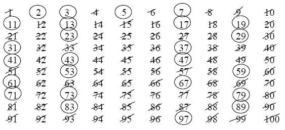
Appendix: The archetypal sieve
The familiar sieve of Eratosthenes is an efficient way to generate
the prime numbers up to a pre-selected bound. Start with the numbers
from 1 to $N$. First cross out the multiples of 2. At each stage
circle the smallest number which has not been crossed out or circled,
and then cross
out all multiples of that number.
Stop when the next number that remains is larger than $\sqrt{N}$.
The numbers which have not been crossed out are the prime numbers
up to $N$.
Using the sieve of Eratosthenes to find all the primes up to $N$ only
requires keeping track of $N$ bits of
information, and uses around $N \log(N)$ operations. To find the primes up to
1 million, it is faster to run the sieve of Eratosthenes
on a computer than
to read those primes from the hard drive.
The sieve of Eratosthenes is efficient
as a practical method for generating the primes, but it is relatively useless as
a theoretical tool. Suppose one wanted to estimate the number of primes
up to $N$. The primes are those numbers which are not crossed out
by the sieve, all we need to do is count how many numbers are crossed
out, and subtract that from $N$. Since some numbers are crossed out
multiple times, we have to use the inclusion-exclusion principle:
\begin{align}
\text{ number of non-primes up to } N =\mathstrut & \text{number crossed out once} \cr
&-\text{number crossed out twice}\cr
&+\text{number crossed out three times}\cr
&- \text{etc.}\nonumber
\end{align}
Unfortunately, estimating the above quantities finds that
the error term is larger than $N$, leaving one with no information at all.
Thus, one must use a more sophisticated sieve to prove results about the primes.