Several examples were considered.
Optimal Stopping and free boundary problems.
Let's consider the following financial market containing a
non-risky asset
![]() , and
, and ![]() risky assets (e.g.
stocks) with prices modeled by a
risky assets (e.g.
stocks) with prices modeled by a ![]() -dimensional diffusion process
S with dynamics
-dimensional diffusion process
S with dynamics
An important problem in finance is the pricing of American
options. Given a reward function ![]() , an American option is a
contract that provides to the owner the right to receive (from the
seller) the amount
, an American option is a
contract that provides to the owner the right to receive (from the
seller) the amount ![]() at any time t if exercised before
some fixed maturity
at any time t if exercised before
some fixed maturity ![]() . This right can be exercised only once
during the period
. This right can be exercised only once
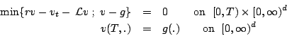
during the period ![]() . The price of this option at time t can
be expressed as the value function associated to the optimal
stopping problem
. The price of this option at time t can
be expressed as the value function associated to the optimal
stopping problem
The associated value function ![]() is the solution of the free
boundary problem
is the solution of the free
boundary problem
Optimal Investment and Hamilton-Jacobi-Bellman equations.
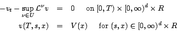
An other important issue in finance is that of optimal investment.
Denoting by ![]() the number of stocks held by a given financial
agent at time t, the associated wealth-process
the number of stocks held by a given financial
agent at time t, the associated wealth-process ![]() has
dynamics given by
has
dynamics given by
Back to the
main index
for Numerical probabalistic methods for high-dimensional problems in finance.