
Matrix Representations
We have seen that linear transformations whose domain and codomain are vector spaces of columns vectors have a close relationship with matrices (Theorem MBLT, Theorem MLTCV). In this section, we will extend the relationship between matrices and linear transformations to the setting of linear transformations between abstract vector spaces.
Definition MR (Matrix Representation) Suppose that $\ltdefn{T}{U}{V}$ is a linear transformation, $B=\set{\vectorlist{u}{n}}$ is a basis for $U$ of size $n$, and $C$ is a basis for $V$ of size $m$. Then the matrix representation of $T$ relative to $B$ and $C$ is the $m\times n$ matrix, \begin{equation*} \matrixrep{T}{B}{C}=\left[ \left.\vectrep{C}{\lt{T}{\vect{u}_1}}\right| \left.\vectrep{C}{\lt{T}{\vect{u}_2}}\right| \left.\vectrep{C}{\lt{T}{\vect{u}_3}}\right| \ldots \left|\vectrep{C}{\lt{T}{\vect{u}_n}}\right. \right] \end{equation*}
Example OLTTR: One linear transformation, three representations.
We may choose to use whatever terms we want when we make a definition. Some are arbitrary, while others make sense, but only in light of subsequent theorems. Matrix representation is in the latter category. We begin with a linear transformation and produce a matrix. So what? Here's the theorem that justifies the term "matrix representation."
Theorem FTMR (Fundamental Theorem of Matrix Representation) Suppose that $\ltdefn{T}{U}{V}$ is a linear transformation, $B$ is a basis for $U$, $C$ is a basis for $V$ and $\matrixrep{T}{B}{C}$ is the matrix representation of $T$ relative to $B$ and $C$. Then, for any $\vect{u}\in U$, \begin{equation*} \vectrep{C}{\lt{T}{\vect{u}}}=\matrixrep{T}{B}{C}\left(\vectrep{B}{\vect{u}}\right) \end{equation*} or equivalently \begin{equation*} \lt{T}{\vect{u}}=\vectrepinv{C}{\matrixrep{T}{B}{C}\left(\vectrep{B}{\vect{u}}\right)} \end{equation*}
This theorem says that we can apply $T$ to $\vect{u}$ and coordinatize the result relative to $C$ in $V$, or we can first coordinatize $\vect{u}$ relative to $B$ in $U$, then multiply by the matrix representation. Either way, the result is the same. So the effect of a linear transformation can always be accomplished by a matrix-vector product (Definition MVP). That's important enough to say again. The effect of a linear transformation is a matrix-vector product.
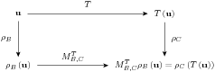
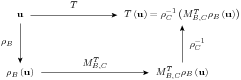
The alternative conclusion of this result might be even more striking. It says that to effect a linear transformation ($T$) of a vector ($\vect{u}$), coordinatize the input (with $\vectrepname{B}$), do a matrix-vector product (with $\matrixrep{T}{B}{C}$), and un-coordinatize the result (with $\vectrepinvname{C}$). So, absent some bookkeeping about vector representations, a linear transformation is a matrix. To adjust the diagram, we "reverse" the arrow on the right, which means inverting the vector representation $\vectrepname{C}$ on $V$. Now we can go directly across the top of the diagram, computing the linear transformation between the abstract vector spaces. Or, we can around the other three sides, using vector representation, a matrix-vector product, followed by un-coordinatization.
Here's an example to illustrate how the "action" of a linear transformation can be effected by matrix multiplication.
Example ALTMM: A linear transformation as matrix multiplication.
We will use Theorem FTMR frequently in the next few sections. A typical application will feel like the linear transformation $T$ "commutes" with a vector representation, $\vectrepname{C}$, and as it does the transformation morphs into a matrix, $\matrixrep{T}{B}{C}$, while the vector representation changes to a new basis, $\vectrepname{B}$. Or vice-versa.
In Subsection LT.NLTFO:Linear Transformations: New Linear Transformations From Old we built new linear transformations from other linear transformations. Sums, scalar multiples and compositions. These new linear transformations will have matrix representations as well. How do the new matrix representations relate to the old matrix representations? Here are the three theorems.
Theorem MRSLT (Matrix Representation of a Sum of Linear Transformations) Suppose that $\ltdefn{T}{U}{V}$ and $\ltdefn{S}{U}{V}$ are linear transformations, $B$ is a basis of $U$ and $C$ is a basis of $V$. Then \begin{equation*} \matrixrep{T+S}{B}{C}=\matrixrep{T}{B}{C}+\matrixrep{S}{B}{C} \end{equation*}
Theorem MRMLT (Matrix Representation of a Multiple of a Linear Transformation) Suppose that $\ltdefn{T}{U}{V}$ is a linear transformation, $\alpha\in\complex{\null}$, $B$ is a basis of $U$ and $C$ is a basis of $V$. Then \begin{equation*} \matrixrep{\alpha T}{B}{C}=\alpha\matrixrep{T}{B}{C} \end{equation*}
The vector space of all linear transformations from $U$ to $V$ is now isomorphic to the vector space of all $m\times n$ matrices.
Theorem MRCLT (Matrix Representation of a Composition of Linear Transformations) Suppose that $\ltdefn{T}{U}{V}$ and $\ltdefn{S}{V}{W}$ are linear transformations, $B$ is a basis of $U$, $C$ is a basis of $V$, and $D$ is a basis of $W$. Then \begin{equation*} \matrixrep{\compose{S}{T}}{B}{D}=\matrixrep{S}{C}{D}\matrixrep{T}{B}{C} \end{equation*}
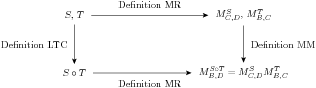
This is the second great surprise of introductory linear algebra. Matrices are linear transformations (functions, really), and matrix multiplication is function composition! We can form the composition of two linear transformations, then form the matrix representation of the result. Or we can form the matrix representation of each linear transformation separately, then multiply the two representations together via Definition MM. In either case, we arrive at the same result.
Example MPMR: Matrix product of matrix representations.
A diagram, similar to ones we have seen earlier, might make the importance of this theorem clearer,
One of our goals in the first part of this book is to make the definition of matrix multiplication (Definition MVP, Definition MM) seem as natural as possible. However, many are brought up with an entry-by-entry description of matrix multiplication (Theorem ME) as the definition of matrix multiplication, and then theorems about columns of matrices and linear combinations follow from that definition. With this unmotivated definition, the realization that matrix multiplication is function composition is quite remarkable. It is an interesting exercise to begin with the question, "What is the matrix representation of the composition of two linear transformations?" and then, without using any theorems about matrix multiplication, finally arrive at the entry-by-entry description of matrix multiplication. Try it yourself (exercise MR.T80).
It will not be a surprise to discover that the kernel and range of a linear transformation are closely related to the null space and column space of the transformation's matrix representation. Perhaps this idea has been bouncing around in your head already, even before seeing the definition of a matrix representation. However, with a formal definition of a matrix representation (Definition MR), and a fundamental theorem to go with it (Theorem FTMR) we can be formal about the relationship, using the idea of isomorphic vector spaces (Definition IVS). Here are the twin theorems.
Theorem KNSI (Kernel and Null Space Isomorphism) Suppose that $\ltdefn{T}{U}{V}$ is a linear transformation, $B$ is a basis for $U$ of size $n$, and $C$ is a basis for $V$. Then the kernel of $T$ is isomorphic to the null space of $\matrixrep{T}{B}{C}$, \begin{equation*} \krn{T}\isomorphic\nsp{\matrixrep{T}{B}{C}} \end{equation*}
Example KVMR: Kernel via matrix representation.
An entirely similar result applies to the range of a linear transformation and the column space of a matrix representation of the linear transformation.
Theorem RCSI (Range and Column Space Isomorphism) Suppose that $\ltdefn{T}{U}{V}$ is a linear transformation, $B$ is a basis for $U$ of size $n$, and $C$ is a basis for $V$ of size $m$. Then the range of $T$ is isomorphic to the column space of $\matrixrep{T}{B}{C}$, \begin{equation*} \rng{T}\isomorphic\csp{\matrixrep{T}{B}{C}} \end{equation*}
Example RVMR: Range via matrix representation.
Theorem KNSI and Theorem RCSI can be viewed as further formal evidence for the \miscref{principle}{Coordinatization Principle}, though they are not direct consequences.
We have seen, both in theorems and in examples, that questions about linear transformations are often equivalent to questions about matrices. It is the matrix representation of a linear transformation that makes this idea precise. Here's our final theorem that solidifies this connection.
Theorem IMR (Invertible Matrix Representations) Suppose that $\ltdefn{T}{U}{V}$ is a linear transformation, $B$ is a basis for $U$ and $C$ is a basis for $V$. Then $T$ is an invertible linear transformation if and only if the matrix representation of $T$ relative to $B$ and $C$, $\matrixrep{T}{B}{C}$ is an invertible matrix. When $T$ is invertible, \begin{equation*} \matrixrep{\ltinverse{T}}{C}{B}=\inverse{\left(\matrixrep{T}{B}{C}\right)} \end{equation*}
By now, the connections between matrices and linear transformations should be starting to become more transparent, and you may have already recognized the invertibility of a matrix as being tantamount to the invertibility of the associated matrix representation. The next example shows how to apply this theorem to the problem of actually building a formula for the inverse of an invertible linear transformation.
Example ILTVR: Inverse of a linear transformation via a representation.
You might look back at Example AIVLT, where we first witnessed the inverse of a linear transformation and recognize that the inverse ($S$) was built from using the method of Example ILTVR with a matrix representation of $T$.
Theorem IMILT (Invertible Matrices, Invertible Linear Transformation) Suppose that $A$ is a square matrix of size $n$ and $\ltdefn{T}{\complex{n}}{\complex{n}}$ is the linear transformation defined by $\lt{T}{\vect{x}}=A\vect{x}$. Then $A$ is invertible matrix if and only if $T$ is an invertible linear transformation.
This theorem may seem gratuitous. Why state such a special case of Theorem IMR? Because it adds another condition to our NMEx series of theorems, and in some ways it is the most fundamental expression of what it means for a matrix to be nonsingular --- the associated linear transformation is invertible. This is our final update.
Theorem NME9 (Nonsingular Matrix Equivalences, Round 9) Suppose that $A$ is a square matrix of size $n$. The following are equivalent.